library(mlr3verse)
library(mlr3extralearners)
# install.packages("mlr3extralearners", repos = "https://mlr-org.r-universe.dev")
bike <- readRDS("bike.rds")
biketask <- as_task_regr(bike, target = "bikers")
splits <- partition(biketask)
tuned_rpf <- auto_tuner(
learner = lrn("regr.rpf", ntrees = 200, max_interaction = 4, nthreads = 2),
tuner = tnr("mbo"),
resampling = rsmp("cv", folds = 3),
terminator = trm("evals", n_evals = 100, k = 10),
search_space = ps(
max_interaction = p_int(2, 10),
splits = p_int(10, 100),
split_try = p_int(1, 20),
t_try = p_dbl(0.1, 1)
),
store_tuning_instance = TRUE,
store_benchmark_result = TRUE
)
tuned_rpf$train(biketask, row_ids = splits$train)Tuning Random Planted Forests with the help of a Random Planted Forest
ml
xai/iml
Lukas Burk 
Abstract
In which we use an untuned model to explain the tuning of a tuned model just to see how it goes.
When we talk about machine learning interpretability methods, we tend to circle back to similar data examples. Partially because there’s a benefit to the familiarity and partially because, well, there’s just a limited number of real-world datasets floating around out there which are both publicly accessible and exhibit some kind of interesting structure that justifies the investigation of, say, third-order interaction effects with some sort of intuitive interpretation.
For IML, the Bikeshare data is one of those popular datasets. We’re using it for a showcase article of the glex R package, and this post is decidedly not about that — but feel free to read the paper (Hiabu, Meyer, et al. 2023).
What this post is actually about is Random Planted Forests (Hiabu, Mammen, et al. 2023, R package on GitHub). I wanted the usage example on the Bikeshare data to be interesting and useful, and since interpretability methods tend to only be as good as the models they’re trying to explain, I first needed a decent model.
So, that’s what this post is about: Tuning rpf, and then using rpf to explain the tuning results.
The Data
We’re using the Bikeshare data as included with the ISLR2 package (originally from the UCI Machine Learning Repository), which I preprocessed and whittled down a little for simplicity’s sake. You can look at the preprocessing steps in the code below, but I’ll skip the dataset exploration as it’s not the focus of this post.
Show preprocessing code
library(data.table)
if (!("ISLR2" %in% installed.packages())) {
  install.packages("ISLR2")
}

data("Bikeshare", package = "ISLR2")

bike <- data.table(Bikeshare)
bike[, hr := as.numeric(as.character(hr))]
bike[, workingday := factor(workingday, levels = c(0, 1), labels = c("No Workingday", "Workingday"))]
bike[, season := factor(season, levels = 1:4, labels = c("Winter", "Spring", "Summer", "Fall"))]
bike[, atemp := NULL]
bike[, day := NULL]
bike[, registered := NULL]
bike[, casual := NULL]

saveRDS(bike, "bike.rds")
Tuning with mlr3
I wrapped the rpf learner into an mlr3 learner for mlr3extralearners, which makes it very convenient to tune. If you’re unfamiliar with the mlr3 ecosystem, well guess who contributed to the now-published mlr3 book available for free online, which you can also buy from your friendly neighborhood dystopian online retailer in fancy tree corpse form.
No judgement.
Mostly.
It’s fine.
Anyway, here’s the code I used, which is fairly standard “wrap learner in AutoTuner and tune the thing with 3-fold cross-validation and a somewhat arbitrary tuning budget using MBO I guess because why not” (WLATT3FCVSATBUMBOIGBWN, as my grampa used to call it).
Ideally, we would evaluate the tuned rpf on the test dataset like this:
pred <- tuned_rpf$predict(biketask, row_ids = splits$test)
pred$score(msr("regr.rmsle"))
…but since I saved the learner with saveRDS() on a different machine and restored it here for use with this post, we only get the error message
Error:
! external pointer is not valid
This is related to rpf using Rcpp modules under the hood, with the takeaway being that at the time of writing I don’t know if there’s a way to serialize and deserialize rpf models for situations like this. This is quite unfortunate, but for the time being we’ll just have to assume that the tuning result is somewhat reasonable. I should have just tuned on the full datasets, but alas, I guess this will have to do now.
Anyways, we extract the tuning archive stored in $archive of the AutoTuner object and convert the MSE we initially tuned with to the RMSE just to get a more manageable range of scores.
library(data.table)
archive <- tuned_rpf$archive$data
archive[, regr.rmse := sqrt(regr.mse)]
The kaggle challenge for this dataset (or a version of it, anyway) evaluates using the RMSLE, which would probably be more appropriate, come to think of it. Putting that one on the “oh well, next time” pile.
Let’s take a look at our scores in relation to our hyperparameter configurations first — one at a time, ignoring any interdependencies.
library(ggplot2)
melt(archive, id.vars = "regr.rmse",
     measure.vars = c("splits", "split_try", "t_try", "max_interaction")) |>
  ggplot(aes(x = value, y = regr.rmse)) +
  facet_wrap(vars(variable), scales = "free_x") +
  geom_point() +
  labs(
    title = "rpf / Bikeshare tuning archive",
    subtitle = "Scores on inner resampling folds",
    x = "Parameter Value", y = "RMSE"
  )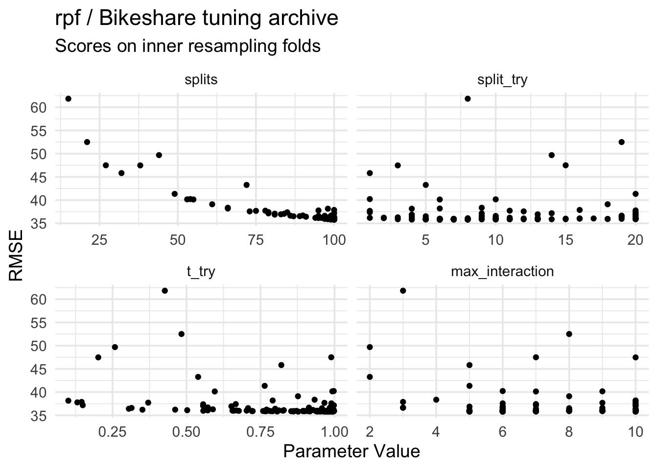
The main thing to note here is that “more splits more good”, while the picture for the other parameters isn’t as clear. Other parameters might interact, and overall it’s not obvious if a parameter is more important than another.
Would be nice if we could somehow functionally decompose the effects of these parameters up to arbitrary ord— oh wait that’s glex, yes, let’s do the glex thing.
Explaining the Tuning Results
Both glex and randomPlantedForest can be installed via r-universe if you can’t be bothered to type remotes::install_github("PlantedML/glex") and/or remotes::install_github("PlantedML/randomPlantedForest"), which I usually can’t:
install.packages(c("glex", "randomPlantedForest"), repos = "https://plantedml.r-universe.dev")library(randomPlantedForest)
library(glex)We then fit another rpf with heuristically picked parameters on the tuning archive, using the RMSE as target and tuning parameters as features. Why not tune rpf “properly” here, you ask? Because I can’t decide whether I want to make this post a recursion joke or not. Also time is finite and I couldn’t be bothered.
rpfit <- rpf(
  regr.rmse ~ splits + split_try + t_try + max_interaction,
  data = archive,
  ntrees = 100,
  splits = 100,
  split_try = 20,
  t_try = 1,
  max_interaction = 4,
  nthreads = 3
)

rpglex <- glex(rpfit, tuned_rpf$archive$data)
Variable Importance
Let’s take a first look at the variable importance scores, calculated as the mean absolute contribution to RMSE of each main- or interaction effect, respectively. The nice thing about this is that we can quantify the relevance of each tuning parameter while fully taking into account any interaction with other parameters, and also quantify the overall relevance of e.g. second-order interactions compared to main effects only.
rpvi <- glex_vi(rpglex)

autoplot(rpvi)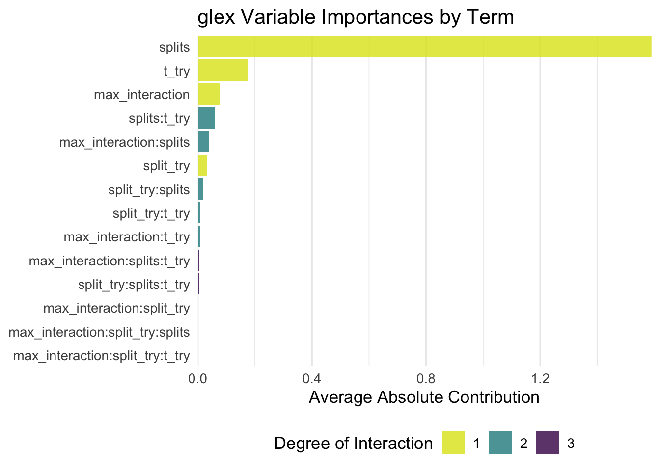
autoplot(rpvi, by_degree = TRUE)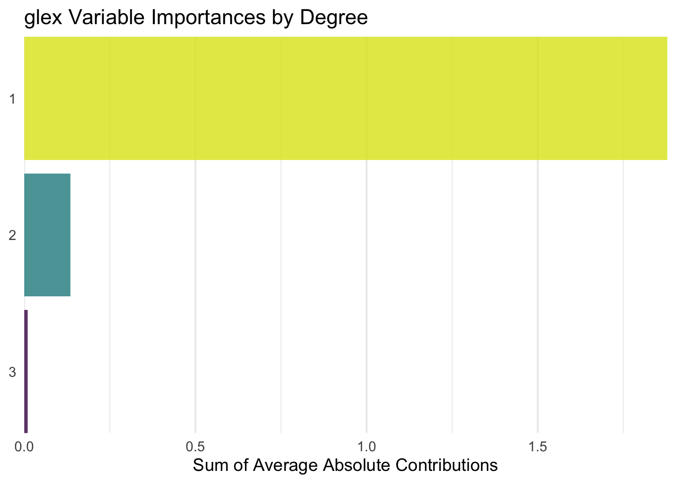
…which definitely could be interesting in some case that is apparently not this one! So yeah.
Turns out splits has by far the largest effect, then we see t_try and max_interaction far behind, while split_try actually turns out to be less influential than its interaction effects with t_try and max_interaction? Okay? Sure, why not. I guess it’s a good thing to see confirmation that, interactions of the 3rd or 4th degree are negligible, and the second-order interactions are not surprising. Also, it confirms that if you only pay attention to one parameter, it should be splits — which is also not particularly surprising, as this parameter controls how long the algorithm runs, meaning that larger values will inevitably lead to better performance than small ones.
Main Effects
Next, let’s see the parameters’ main effects, meaning the difference from the average predicted value (intercept) across the observed parameter values.
Note the varying y-axis scales — they’re kind of important here.
library(patchwork)
p1 <- autoplot(rpglex, "splits")
p2 <- autoplot(rpglex, "t_try")
p3 <- autoplot(rpglex, "max_interaction")
p4 <- autoplot(rpglex, "split_try")

(p1 + p2) / (p3 + p4)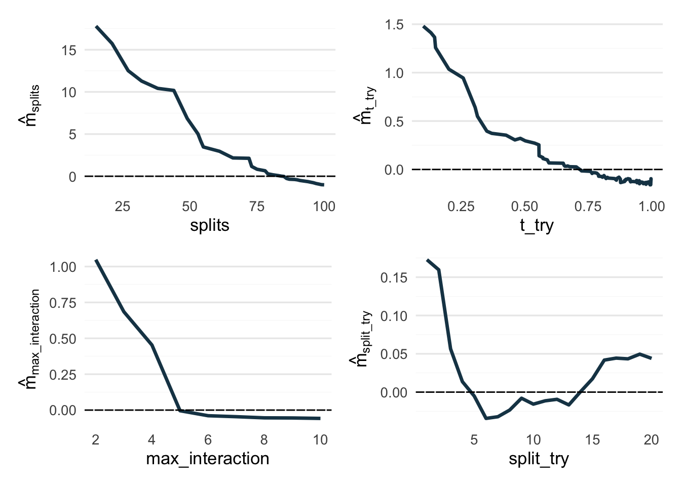
So, in short: splits wants to be large, t_try wants to be close to 1, max_interaction most likely also wants to be large up to some point, and split_try is pulling a ¯\_(ツ)_/¯ on us.
Fair enough.
Interaction Effects
We can also take a look at the two largest interaction effects, splits:split_try and splits:t_try, but to be quite honest I’m not sure what to make of these plots except for how they illustrate in which direction MBO has taken the tuning process (large values for splits and t_try).
autoplot(rpglex, c("splits", "split_try")) +
autoplot(rpglex, c("splits", "t_try"))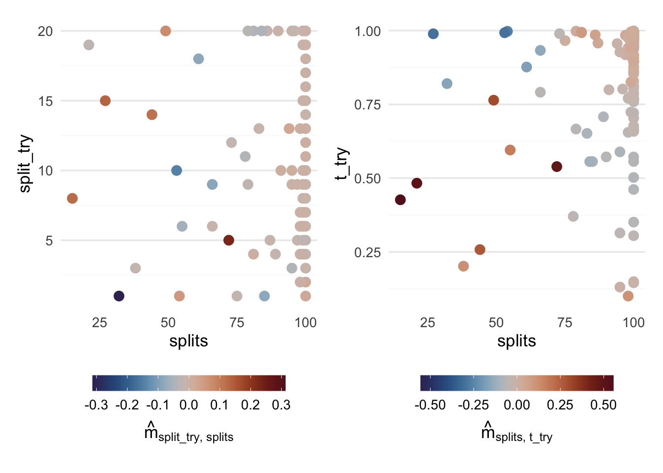
Finally, here’s the final parameter configuration that “won”, meaning these are the parameters I’ll be using to fit an rpf to the Bikeshare data in a new version of the glex vignette:
tuned_rpf$tuning_result[, c("splits", "split_try", "t_try", "max_interaction")] splits split_try t_try max_interaction
<int> <int> <num> <int>
1: 100 6 0.9422986 6c(rmse = sqrt(tuned_rpf$tuning_result$regr.mse)) rmse
35.79528 …And thanks to glex, I guess I have a better intuition for these parameters now? Is that how it works? Let’s say it does.
I’m not entirely sure how much I want to trust these results or want to make generalizations based off of them (I don’t), but the underlying principle seems quite useful to me. rpf is still a fairly young method and gaining intuition for its parameters like this seems neat.
Conclusion
The key takeaway for the Bikeshare tuning is that:
splitswants to be large.t_trywants to be close to 1.- Setting
max_interactionto 5 or greater is only going to make you wait for the result longer. split_tryis also a parameter that exists. Idunno maybe just wing it with that boi and be done with it.
Turns out it wasn’t particularly eye-opening to take a look at parameter interactions, but oh well. Better to have decomposed and not needed it than to never decompose at all. Or something.
References
Hiabu, Munir, Enno Mammen, and Joseph T. Meyer. 2023. Random Planted Forest: A Directly Interpretable Tree Ensemble. https://arxiv.org/abs/2012.14563.
Hiabu, Munir, Joseph T. Meyer, and Marvin N. Wright. 2023. “Unifying Local and Global Model Explanations by Functional Decomposition of Low Dimensional Structures.” In Proceedings of the 26th International Conference on Artificial Intelligence and Statistics, edited by Francisco Ruiz, Jennifer Dy, and Jan-Willem van de Meent, vol. 206. Proceedings of Machine Learning Research. PMLR. https://proceedings.mlr.press/v206/hiabu23a.html.